We investigate optimal decision-making under endogenous distribution shifts with latent dynamics. These shifts arise from the dynamic interaction of a decision-maker and an evolving distribution. We present a motivating example in the domains of opinion dynamics.

Aligned with this motivating example, here we explore general stochastic optimization with endogenous distribution shifts arising from the interaction between a decision-maker and a dynamic distribution, see (1) for an illustration. This setup involves several major challenges. First, the largely unknown distribution dynamics exclude an offline strategy based on the exact (re)formulation of the decision-making problem. Second, while the paradigm of repeated sampling and retraining in performative prediction facilitates adaptation (see (1.3)), achieving optimality beyond performative stability requires anticipating how the decision affects the distribution and applying proactive adjustments. Finally, the dynamic setup restricts us from sampling from the steady-state distribution corresponding to the decision, which is the very distribution we care about while evaluating the overall performance. In this paper, we will address these challenges by developing and analyzing an online stochastic algorithm tailored to this dynamic setting.

We are motivated by applications where a decision-maker drives a constantly evolving distribution and aims to optimize the distribution-level performance. We formulate a decision-dependent stochastic problem featuring endogenous distribution shifts with latent dynamics. For this general and dynamic setting, we adopt a distributional perspective at the intersection of stochastic optimization, nonlinear control, and metric probability spaces and present the following contributions.

• We characterize the distribution shift via the contracting coefficient of distribution dynamics and the change of decisions. To this end, we use as the main metric the Wasserstein distance [5] between the current distribution and its steady-state distribution induced by the decision. This metric plays a similar (albeit not necessarily the same) role as a Lyapunov function in control theory [24]. Although the exact value of such a Wasserstein distance can be elusive, the recursive inequality related to this metric sheds light on the dynamic evolution of the distribution.
• We propose an online stochastic algorithm that leverages samples from the current distribution and takes into account the composite structure of the problem due to dynamics. The iterative update direction consists of two terms. One term focuses on adaptation, and the most recent samples are exploited to adjust decisions. The other term actively shapes future distributions by anticipating the sensitivity of the distribution with respect to the decision, thereby informing optimal decision-making. Notably, our algorithm does not resort to a world model of the dynamic distribution; instead, the only adopted information is the so-called sensitivity, which is easily learnable in many scenarios.
• We establish optimality guarantees of the proposed algorithm in a nonconvex setting. In the face of dynamics and the composite structure, the convergence measure (i.e., the expected second moment of gradients) enjoys a favorable \( \mathcal{O}(1/\sqrt{T})\) rate, where \( T\) is the total number of iterations. This rate is as sharp as that of stochastic gradient descent for static nonconvex problems without decision dependence. Further, we provide high-probability convergence guarantees for a single run of the proposed algorithm. The key insight is to synthesize the coupled evolution of the aforementioned Wasserstein metric and the convergence measure, which correspond to the dynamic distribution and the iterative algorithm, respectively.
• We quantify the finite-sample generalization performance. We explore how the decisions obtained based on an empirical distribution with finite samples will generalize to the original distribution-level problem. We demonstrate that the generalization measure scales polynomially with the number of samples and the number of iterations, as well as polylogarithmically with the inverse of the failure probability. These results are built on the measure concentration argument and the characterization of the distribution shift, illustrating the benefits of our distributional perspective.
• We illustrate the aforementioned results with practical examples, where an opportunistic party maximizes the affinity of a polarized dynamic population, and a recommender optimizes performance by interacting with a user. In the first setup, the population is modeled as a continuous distribution, whereas in the second example, the user is represented by a discrete distribution evolving in the probability simplex. We demonstrate that respecting the composite problem structure due to decision dependence is crucial for achieving fast convergence and improved optimality.

A multitude of works investigate the roles of distribution shifts and decision dependence in machine learning, optimization, and control. We provide a concise review of their setups and foci.

In applications, data-generating distributions can change because of various factors, e.g., non-stationary environment, unknown covariate shifts, and adversarial effects. There are two predominant strategies for addressing distribution shifts. One strategy pursues robustness against potential perturbations to distributions. This falls under the umbrella of distributionally robust optimization [25, 26] and is achieved by optimizing the worst-case cost over a so-called ambiguity set, i.e., the family of distributions that are close to the true distribution under certain metrics. Further, in two-stage stochastic programming, the first-stage decision may change the uncertain distribution in the second stage, thereby producing a decision-dependent ambiguity set [1]. Tractable reformulations are derived in [2, 3] to disentangle this dependence and obtain robust solutions.

In the face of constantly evolving distributions, a less conservative and more active strategy is to seek adaptation. Specifically, online stochastic optimization investigates an iterative loop whereby a decision-maker commits a decision, receives samples from a dynamic distribution as feedback [13, 14], and then generates a new decision. Such an online framework is versatile and particularly suitable to tackle exogenous distribution shifts, which are out of the influence of a decision-maker. Nonetheless, in terms of optimization subject to endogenous distribution shifts caused by decisions (see also the beginning of (1)), unique phenomena (e.g., the existence of equilibria and stability issues) arise, requiring tailored methods for this closed-loop setting. We delineate some representative works as follows.

Performative prediction studies optimization under decision-dependent distributions [15, 16]. A canonical example is strategic classification, where an individual deliberately modifies her feature in reaction to the deployed classifier, thereby gaining a more favorable classification result. Such endogenous distribution shifts are usually formalized as static distribution maps parameterized by decisions. This setup leads to a novel equilibrium notion termed performative stability, meaning the decision optimizes the objective given the specific distribution it induces. Through repeated sampling and retraining, various stochastic algorithms converge to performatively stable points [27, 28]. A stronger solution concept is performative optimality, requiring that the decision and the induced distribution together lead to an optimal objective value. Convergence to performatively optimal points is achieved with additional structural assumptions on the distribution map, e.g., it belongs to a linear location-scale family [29, 30, 31, 32] or an exponential family [33]. As a general, elegant, and tractable framework, performative prediction admits numerous extensions, including network scenarios with cooperative [34] or competing agents [31, 35], time-varying objectives [36, 37], saddle point minimax problems [38], and coupling constraints [32].

Our work is closely related to stateful performative prediction, which captures historical dependence and considers an evolving distribution that gradually settles at the stationary distribution map. Models of historical dependence include geometrically ergodic Markov chains [39] and geometric decay responses in the form of linear mixture [40, 41]. With Lipschitz distribution shifts assumed in the first place, the algorithms therein converge to performatively stable (albeit not necessarily optimal) points. In contrast, we formalize a decision-dependent distribution shift featuring a broad class of nonlinear dynamics mixing continuous decisions and state distributions. Moreover, we explicitly characterize the distribution shift through the Wasserstein metric [5] and link this shift with dynamics parameters and the change of decisions. We further establish convergence to locally optimal solutions given a nonconvex objective function involving the decision-dependent structure.

Along the line of performative decision-making, some recent works study the role of dynamics in the decision-dependent problem setup. Performative reinforcement learning [42] handles transition probability and reward functions relying on the deployed policy and finds a stable policy given cumulative rewards. Performative control in [59] addresses linear dynamics with policy-dependent state transition matrices and seeks a performatively stable control solution as a linear combination of states and disturbances. The framework of [4] represents the dynamics of a strategic population via a gradient flow in the Wasserstein space. The interconnection of this strategic population and a decision-maker results in coupled partial differential equations, which admit asymptotic convergence to optimal solutions for convex (or concave) energy functionals. In contrast, we characterize the distribution shift represented by general nonlinear dynamics. Furthermore, we offer insights into anticipating the sensitivity of the distribution shift, taking into account the composite structure due to dynamics in the algorithmic design, and achieving (locally) optimal decision-making in the context of nonconvex objectives. The incorporation of anticipating sensitivity to actively shape distributions is the distinguishing feature of our algorithm compared to the aforementioned performative methods.

Mean-field formulation abstracts the mutual influence in a vast homogeneous population by the interaction between a representative individual and an average density, i.e., the mean field [43]. This abstraction facilitates approximately solving an otherwise intractable multi-agent problem, wherein the joint states and actions may grow exponentially with the number of agents. The solutions to mean-field games or control are characterized by two coupled equations, namely, a forward equation for the evolving mean-field distribution and a backward equation associated with the individual value function. Classical approaches rely on the full knowledge of population dynamics and work under restrictive assumptions [21]. A recent trend is to apply reinforcement learning to learn models of dynamics [44], value functions, or policy functions [45], thereby obtaining Nash equilibrium or socially optimal policies. Different from the mean-field formulation, we examine a simplified case where individuals do not interact with one another. Nevertheless, we provide the following new insights. First, we require less information or learning effort related to distribution dynamics. Rather than constructing well-calibrated models, we only access steady-state sensitivity matrices corresponding to dynamics, which are easily learnable, see (2.2). Second, we explicitly characterize the distribution shift via dynamics parameters and the change of decisions. Finally, instead of analyzing a cumulative cost and a state-feedback policy, we seek optimal steady-state performance and a general decision vector. For the generic setting with nonconvex objectives and nonlinear dynamics, we quantify the local optimality of the obtained solutions.

Control in probability spaces addresses the formulation where the state of a system is a probability measure instead of a Euclidean vector [46]. This formulation facilitates the characterization of the evolving uncertainties in a system or the collective behavior of a population, both of which are intrinsically modeled via probability distributions [47, 18]. A typical example is distribution steering, i.e., driving the state distribution from an initial density to a target density in finite time with minimum energy control [46]. In this regard, tractable control strategies cross-fertilize insights from control theory (e.g., linear state-feedback structures) and optimal transport [e.g., transport map calculations, 5]. In contrast, we search for an optimal decision vector rather than a state feedback control policy. Further, we do not aim for a specific final distribution. Instead, we hope the decision, together with the distribution induced through the nonlinear dynamics, will lead to an optimal steady-state behavior.

In a broader context, our work aligns with feedback optimization [48, 49], which implements optimization iterations as a feedback controller, thereby regulating the steady-state behavior of a dynamical system. Nonetheless, in this paper we are concerned with distribution-level characterizations in a metric space of probability measures, which is drastically different from the system-theoretic analysis of feedback optimization in Euclidean space.

In summary, we capture the distribution shift arising from the dynamic evolution of a distribution driven by a decision-maker. Such dynamics are represented by a broad class of nonlinear equations encompassing continuous states and decisions. We propose and characterize an online stochastic algorithm that respects the composite problem structure due to dynamics, regulates the distribution flow, and yields locally optimal solutions to the overall nonconvex problem featuring decision dependence.

The remainder of this paper is structured as follows. (2) introduces preliminaries of the metric probability space and formulates the stochastic optimization problem involving dynamic decision-dependent distributions. (3) presents the intuitions and design of our online stochastic algorithm. In (4), we characterize the distribution dynamics and establish guarantees on the optimality and generalization performance of the proposed algorithm. (5) showcases an application in affinity maximization with a polarized population following (1), as well as another case study in a recommender system context involving discrete distributions. Finally, (6) concludes this paper and discusses future directions. All proofs are provided in the appendix.

We review the background of a metric probability space and refer the readers to [5] for more details. Let \( \mathcal{P}(\mathbb{R}^m)\) be the space of Borel probability distributions on \( \mathbb{R}^m\) . Let \( \mathcal{P}_1(\mathbb{R}^m) \triangleq \big\{\mu \in \mathcal{P}(\mathbb{R}^m): \int_{\mathbb{R}^m} \|x\| \,\mathrm{d} \mu(x) < \infty \big\}\) be the space of distributions with finite absolute moments. The Dirac mass at point \( x \in \mathbb{R}^m\) is denoted by \( \delta_x\) , i.e., for any Borel set \( A \subseteq \mathbb{R}^m\) , \( \delta_x(A) = 1\) if \( x \in A\) and \( \delta_x(A) = 0\) otherwise. We use \( X \sim \mu\) to indicate that a random variable \( X\) is distributed according to \( \mu\) . The convolution of two distributions \( \mu, \nu \in \mathcal{P}_1(\mathbb{R}^m)\) is denoted by \( \mu * \nu\) . Specifically, if two random variables \( X\) and \( Y\) are independent and distributed according to \( \mu\) and \( \nu\) , respectively, then \( X+Y \sim \mu * \nu\) . The pushforward of a distribution \( \mu\) via a Borel map \( f: \mathbb{R}^{r} \to \mathbb{R}^m\) is represented by \( f_{\#}\mu\) , where \( (f_{\#} \mu)[A] \triangleq \mu[f^{-1}(A)]\) for every Borel set \( A \subseteq \mathbb{R}^m\) . In fact, if \( X \sim \mu\) , then \( f(X) \sim f_{\#} \mu\) . The identity map is \( \mathopen{}\mathrm{Id}\) .

Let \( \|z\|_P = \sqrt{z^\top P z}\) denote the weighted norm of a vector \( z \in \mathbb{R}^m\) , where \( P \in \mathbb{R}^{m\times m}\) is positive definite. Consider a metric space \( (\mathbb{R}^m, c)\) endowed with a continuous metric \( c : \mathbb{R}^m \times \mathbb{R}^m \to \mathbb{R}_{\geq 0}\) . Typical examples of \( c\) include the Euclidean distance \( c(x,y) = \|x-y\|\) , the weighted distance \( c(x,y) = \|x-y\|_P\) , and other distances defined by composite norms, where \( x,y \in \mathbb{R}^m\) . The type-\( 1\) Wasserstein distance \( W_1(\mu,\nu)\) between two distributions \( \mu, \nu \sim \mathcal{P}_1(\mathbb{R}^m) \) on \( (\mathbb{R}^m, c)\) is

where \( \Gamma(\mu,\nu)\) is the set of all joint distributions (i.e., couplings) with marginals \( \mu\) and \( \nu\) , see [5, Definition 6.1]. Intuitively, the Wasserstein distance is the minimum cost of transporting \( \mu\) onto \( \nu\) , where the cost of moving a unit mass from \( x\) to \( y\) is \( c(x,y)\) , and the available transport plan is represented by \( \gamma\) . The Wasserstein distance is a flexible and quantitative measure of the discrepancy between distributions, particularly when they have disjoint supports, such as when one distribution is continuous and the other is discrete.

We generalize the motivating case study in (1) and consider the following distribution dynamics with continuous states

In (3), \( p_k \in \mathbb{R}^m\) is a random state at time \( k\) distributed according to \( \mu_k\) , i.e., \( p_k \sim \mu_k\) . The initial state \( p_0\) satisfies the distribution \( \mu_0 \in \mathcal{P}_1(\mathbb{R}^m)\) . Further, \( u \in \mathbb{R}^n\) is a decision (or an input) that influences each random state, and \( d \in \mathbb{R}^r\) following the distribution \( \mu_d \in \mathcal{P}_1(\mathbb{R}^r)\) is an exogenous input that remains constant during iterations. For instance, \( d\) can be a bias term (similar to the initial position in (1)), a disturbance, or a random parameter in a model of \( f\) . Each pair \( (p_0,d)\) is independently drawn from the joint distribution \( \alpha\) , and the first and the second marginals of \( \alpha\) are \( \mu_0\) and \( \mu_d\) , respectively. For instance, if \( p_0\) and \( d\) as well as \( \mu_0\) and \( \mu_d\) are the same (c.f. (1)), then \( \alpha = ( \mathopen{}\mathrm{Id}, \mathopen{}\mathrm{Id})_{\#} \mu_0\) ; if \( p_0\) and \( d\) are independent, then \( \alpha\) is the product measure \( \mu_0 \times \mu_d\) .

The distribution dynamics (3) feature decision dependence, in that the evolution of the distribution \( \mu_k\) is driven by the decision \( u_k\) . The status of this distribution will in turn determine the optimal decision for an optimal distribution-level behavior. Before we present the formal problem description, we specify some properties related to the dynamics (3). All these properties serve the purpose of characterization and analysis. Our online algorithm does not resort to the model \( f\) of the distribution dynamics; rather, it leverages samples and certain learnable sensitivities related to (3).

(1) implies that the dynamics (3) are contracting in \( p\) with respect to the weighted norm \( \|\cdot\|_P\) . The existence and conditioning of \( P\) (i.e., the so-called contraction metric) are known for incrementally exponentially stable nonlinear dynamics [50]. Based on the Lipschitz conditions of \( f\) , the Banach contraction theorem ensures that for a fixed input \( u\) (i.e., \( u_kū,\forall k \in \mathbb{N}_{+}\) ) and a specific exogenous input \( d\) , the dynamics (3) admit a unique steady state \( p_\textup{ss} = h(u,d)\) satisfying \( p_\textup{ss} = f(p_\textup{ss},u,d)\) . We can further establish that \( h\) is \( L_hû\) -Lipschitz in \( u\) and \( L_h^d\) -Lipschitz in \( d\) with respect to \( \|\cdot\|\) , where \( L_hû = L_fû\sqrt{\lambda_{\max}(P)/\lambda_{\min}(P)}/(1-L_f^p)\) and \( L_h^d = L_f^d\sqrt{\lambda_{\max}(P)/\lambda_{\min}(P)}/(1-L_f^p)\) , see the parametric contraction mapping principle [51, Theorem 1A.4] and also (5) in (A). The Lipschitz continuity of \( \nabla_u h(u,d)\) (i.e., the so-called sensitivity matrix) can be satisfied when \( f\) has bounded Hessians. As we will see in (2) below, stable linear dynamics naturally satisfy (1).

From a distribution-level perspective, all the steady-state samples \( p_\textup{ss}\) satisfy the following distribution \( \mu_\textup{ss}(u)\) that depends on \( u\) and \( \mu_d\)

where \( h(u,\cdot)_{\#} \mu_d\) denotes the pushforward of the distribution \( \mu_d\) via a Borel map \( h(u,\cdot): \mathbb{R}^r \to \mathbb{R}^m\) parameterized by the decision \( u\) . Let \( \nabla_u h(u,d) \in \mathbb{R}^{n\times m}\) be the steady-state sensitivity matrix of \( p_\textup{ss} = h(u,d)\) with respect to the decision \( u\) . It follows from the implicit function theorem [51, Theorem 1B.1] that

which holds in an open neighborhood of \( (u,d)\) . The sensitivity \( \nabla_u h(u,d)\) quantifies the rate of change of the steady-state sample \( p_\textup{ss}\) with respect to the decision \( u\) . While (5) may seem daunting at first glance, the sensitivity can be simplified in various scenarios. For instance, when the dynamics (3) are linear, the corresponding sensitivity becomes a constant matrix, see (2) below. If the exogenous input \( d\) is additive in (3), then the detailed form of (5) no longer involves \( d\) . More broadly, apart from invoking (5) based on the related knowledge of dynamics and parameters, we can exploit recursive estimation or identification techniques to construct (approximate) sensitivities, see [49, Sec. 3.3.1] in the context of widely adopted feedback optimization methods. Such a learnable sensitivity is the only model information on (3) used in our online algorithm. All the characterizations in (1) are for the sake of analysis, and the full world model (i.e., \( f\) ) of the distribution dynamics is not required.

In the following example, we review an important special case of (3), where the dynamics function is linear. We will see how (1) is justified and provide explicit expressions of the distribution \( \mu_k\) at time \( k\) and the steady-state distribution \( \mu_\textup{ss}(u)\) .

We aim to find a decision \( u\) that optimizes the steady-state behavior of the dynamic distribution (3):

where \( \mu_\textup{ss}(u)\) is the steady-state distribution of (3) induced by \( u\) , see also (4). Let the reduced objective function of problem (6) be denoted by

The decision-dependent problem (6) formalizes the steady state of the closed loop illustrated by (1) in (1.1). This problem is relevant in many scenarios with a vast population or intrinsic uncertainties, e.g., voting and recommender systems.

Problem (6) involves several major challenges in terms of the nonconvex objective and the unknown dynamics underlying the decision-dependent distribution.

• First, the distribution dynamics (3) induce the steady-state distribution \( \mu_\textup{ss}(u)\) and further bring about a composite structure in problem (6). Even for a convex function \( \Phi\) , since the steady-state map \( h(u,d)\) is nonlinear, the overall objective \( \tilde{\Phi}(u)\) can be nonconvex.
• Another challenge originates from the unknown distribution dynamics, which render the structure of decision dependence elusive and preclude an offline numerical scheme based on the exact (re)formulation of problem (6).
• Finally, we cannot directly sample from the steady state distribution \( \mu_\textup{ss}(u)\) unless we wait sufficiently long, because the distribution \( \mu_k\) is constantly changing with time \( k\) and eventually approaches \( \mu_\textup{ss}(u_k)\) .

To overcome the above challenges, we will propose an online stochastic algorithm in (3) that samples from the current distribution \( \mu_k\) and regulates the distribution shift by anticipating its sensitivity with respect to the decision.

We focus on steady-state performance due to relevance, generality, and tractability. First, in many problems an optimal steady state matters more than transients, with the latter often not even being modeled, see for instance in many case studies where feedback optimization or performative prediction is applied. This setup will also allow us to circumvent the need for model knowledge by exploiting distribution sensitivity, which is easier to learn. Second, if we analyze the behavior of a stable and dynamic distribution over a sufficiently long horizon, then the average performance metric (i.e., the cumulative objective values divided by the number of iterations) essentially converges to the steady-state objective. Finally, in this context we can go beyond the assumptions and policy classes considered in the mean-field literature [21] and establish provable guarantees for continuous decision vectors given a broad class of nonlinear dynamics and nonconvex objective functions. Specifically, we make the following assumptions on the objective.

(2) requires a well-defined expectation function, which is common in stochastic optimization [see 12, Section 9.2.5] and can be satisfied, e.g., when for each \( u\) , \( \Phi(u,h(u,d))\) is dominated by an integrable function of \( d\) . The smoothness condition is also standard [see 52] and holds, e.g., when for every stochastic sample \( p_\textup{ss}=h(u,d)\) , the objective \( \Phi(u,p_\textup{ss}) = \Phi(u,h(u,d))\) is \( L_{\tilde{\Phi}}\) -smooth and the second moment of \( L_{\tilde{\Phi}}\) is bounded. The requirement that the partial gradients are Lipschitz in the random variable \( p\) is related to (though not the same as) the joint smoothness property used in performative prediction [15, 27]. Moreover, the condition that \( \tilde{\Phi}(u)\) is bounded below implies that problem (6) admits a finite optimal value \( \tilde{\Phi}^* \in \mathbb{R}\) .

(3) is similar to [12, Eq. (9.130)]. It is a sufficient condition for the interchangeability of the expectation and gradient operators, see [12, Theorem 9.56] and also (8) in (3.1) below. If the function \( \Phi(u,h(u,d))\) is Lipschitz continuous in \( u\) , then (3) holds naturally.

We provide the intuition of constructing appropriate stochastic gradients for online decision-making as per (6). Ideally, we aim to obtain the gradient of the objective \( \tilde{\Phi}\) at \( u_k\) , i.e.,

where (a.1) leverages interchangeability of the expectation and gradient operators thanks to (3), see also [12, Theorem 9.56]; (a.2) uses the law of the total derivative; (a.3) involves expectation with respect to the joint distribution \( \gamma_\textup{ss}(u_k) \triangleq (h(u_k,\cdot), \mathopen{}\mathrm{Id})_{\#} \mu_d\) of the steady-state variable \( p \sim \mu_\textup{ss}(u_k) = h(u_k,\cdot)_{\#} \mu_d\) and the exogenous input \( d \sim \mu_d\) .

However, the exact gradient \( \nabla \tilde{\Phi}(u_k)\) can be difficult to calculate for two reasons. First, it involves the expectation with respect to the random variable \( p\) , although in practice we can only access finite samples of the distribution. Second, since each sample needs a few iterations to approach its steady state, the steady-state distribution \( \mu_\textup{ss}(u_k)\) of \( p\) corresponding to the decision \( u_k\) is unavailable at the current time \( k\) .

To address these issues, we use samples drawn from the current distribution \( \gamma_k\) to construct a mini-batch stochastic gradient, thereby informing decision-making. The intuition is that \( \gamma_k\) , as reflected by these samples, serves as a reasonable proxy for the steady-state distribution \( \gamma_\textup{ss}(u_k)\) , provided that neighboring decisions (i.e., \( u_{k-1}\) and \( u_k\) ) are close and the iteration counter \( k\) is large. Consequently, the expected gradient involving \( \gamma_k\) also becomes a close approximation of the exact gradient \( \nabla \tilde{\Phi}(u_k)\) entailing \( \gamma_\textup{ss}(u_k)\) . We will formalize this intuition in (4.1).

Guided by the aforementioned intuition, our online stochastic algorithm for solving problem (6) is

where \( \eta > 0\) is a constant step size, \( k\) is the iteration counter, and \( \widehat{\nabla}_\textup{{mb}}^{k} \tilde{\Phi}(u_k)\) is a stochastic gradient based on mini-batches, i.e.,

In (11), \( n_\textup{{mb}} \in \mathbb{N}_{+}\) is the size of the mini-batch, and \( \nabla_u h(u_k,d^i)\) is the steady-state sensitivity of \( p^i_\textup{ss}\) with respect to the decision \( u_k\) . Such a sensitivity admits various simplifications and can often be learned from data in practice, see the discussion in (2.2). For instance, the sensitivity is a constant matrix given linear dynamics and does not involve \( d^i\) if the exogenous input is additive. Further, \( p_k^1, …, p_k^{n_\textup{{mb}}}\) are samples drawn from the transient distribution \( \mu_k\) at time \( k\) . These samples rely on the decisions owing to the dynamics (3), thereby causing a composite structure in the objective \( \Phi(u,p)\) .

In essence, the mini-batch stochastic gradient (11) is a finite-sample approximation of

i.e., the approximate expected gradient at \( u_k\) when \( p\) and \( d\) satisfy the joint distribution \( \gamma_k\) . Specifically, \( \gamma_k = (f^{(k)}(x,y),y)_{\#}\alpha(x,y)\) denotes the pushforward of \( \alpha\) in (3). Further, \( f^{(k)}(p_0,d)\) is the value of \( p_k\) given a pair of the initial state \( p_0\) and the exogenous input \( d\) sampled from the joint distribution \( \alpha\) , a sequence of decisions \( (u_i)_{i=1,…,k}\) , and the dynamics (3). That is, \( f^{(k)}: \mathbb{R}^m \times \mathbb{R}^r \to \mathbb{R}^m\) is a map parameterized by \( u_1,…,u_k\) . We define the special case \( f^{(0)}(p_0,d)\) as \( p_0\) . We will show in (4) that with suitable algorithmic parameters, \( \widehat{\nabla}_\textup{{mb}}^{k} \tilde{\Phi}(u_k)\) and \( \widehat{\nabla}^k \tilde{\Phi}(u_k)\) are close to \( \nabla \tilde{\Phi}(u_k)\) , enabling the stochastic algorithm (10) to yield (locally) optimal solutions.

The mini-batch stochastic gradient \( \widehat{\nabla}_\textup{{mb}}^{k} \tilde{\Phi}(u_k)\) involves two terms. Term ➀ in (11) leverages the current sample \( p_k^i\) to construct a partial gradient with respect to \( u\) . Term ➁ in (11) anticipates how the decision \( u_k\) will influence the sample \( p\) (and in turn the objective) and uses this link for achieving optimality. As explained in (3.1), these two terms result from the aforementioned composite structure of \( \Phi(u,p)\) and the law of the total derivative. While the update rule (10) seems obvious from our presentation, most related online methods do not use an anticipating term as ➁ in (11), as discussed in (1.3).

Let \( \mathcal{F}_k\) be the \( \sigma\) -algebra generated by the random variables \( \widehat{\nabla}_\textup{{mb}}^{0} \tilde{\Phi}(u_0), …, \widehat{\nabla}_\textup{{mb}}^{k}\tilde{\Phi}(u_k)\) . Hence, the decision \( u_k\) is measurable with respect to \( \mathcal{F}_{k-1}\) . We make the following assumption on the variance of the stochastic gradient constructed from an individual sample. For a stochastic vector \( \xi \in \mathbb{R}^n\) , we define its variance as \( \operatorname{Var} [\xi] \triangleq \mathrm{ \mathbb{E} }\left[\|\xi - \mathrm{ \mathbb{E} }[\xi]\|^2\right] = \mathrm{ \mathbb{E} }[\|\xi\|^2] - \left\|\mathrm{ \mathbb{E} }[\xi]\right\|^2\) .

(4) is a standard and relatively weak statement that the variance of the stochastic gradient is restricted [52]. It implies that this variance can be nonzero at the point where \( \widehat{\nabla}^k \tilde{\Phi}(u_k)\) equals zero and grows at most quadratically in the norm of \( \widehat{\nabla}^k \tilde{\Phi}(u_k)\) .

Given the dynamics (3) and independent pairs \( (p_0^1,d^1), …, (p_0^{n_\textup{{mb}}},d^{n_\textup{{mb}}})\) of initial states and exogenous inputs, when conditioned on \( \mathcal{F}_{k-1}\) , the samples \( p_k^1, …, p_k^{n_\textup{{mb}}}\) collected at time \( k\) are still independent. Building on this observation, we specify some key properties of the mini-batch gradient \( \widehat{\nabla}_\textup{{mb}}^{k} \tilde{\Phi}(u_k)\) in the lemma below.

The distribution dynamics (3) bring about constant shifts of the joint distribution \( \gamma_k\) . We characterize such distribution shifts through the lens of the Wasserstein distance. Specifically, we focus on the behavior of \( W_1(\gamma_k,\gamma_\textup{ss}(u_k))\) , i.e., the Wasserstein distance between the joint distribution \( \gamma_k\) at time \( k\) and the joint steady-state distribution \( \gamma_\textup{ss}(u_k)\) induced by the decision \( u_k\) .

Throughout this section, we consider the space \( (\mathbb{R}^{m+r},c)\) endowed with the metric

where \( p,p' \in \mathbb{R}^m, d,d' \in \mathbb{R}^r\) , and \( \|\cdot\|_P\) is the weighted norm. Then, \( W_1(\gamma_k,\gamma_\textup{ss}(u_k))\) is defined by

where \( (p,d)\) and \( (p',d')\) are distributed according to \( \gamma_k\) and \( \gamma_\textup{ss}(u_k)\) , respectively.

The following lemma gives an upper bound on the Wasserstein distance \( W_1(\gamma_k,\gamma_\textup{ss}(u_k))\) and establishes a related recursive inequality. It is built on the properties of the pushforward operation induced by Borel maps, see [58, Proposition 3]. Recall that \( L_f^p\) is the Lipschitz constant of the dynamics function \( f\) with respect to \( p\) under \( \|\cdot\|_P\) , and that \( L_hû\) is the Lipschitz constant of the steady-state map \( h\) of (3) with respect to \( u\) under \( \|\cdot\|\) , see (1) and the discussion below. Further, \( \lambda_{\max}(P) > 0\) is the maximum eigenvalue of the positive definite matrix \( P\) , and \( f^{(k)}(p_0,d)\) denotes the value of \( p_k\) given a pair \( (p_0,d) \sim \alpha\) and past decisions, see the paragraph below (12) in (3.1).

(2) characterizes the behavior of \( W_1(\gamma_k,\gamma_\textup{ss}(u_k))\) through the evolution of the upper bound \( V_k\) . Specifically, this upper bound exhibits perturbed contraction (16.b), where the contraction coefficient is \( L_fû \in (0,1)\) , and the perturbation term is proportional to the difference of consecutive inputs. If the inputs are kept fixed (i.e., \( u_k = u,\forall k \in \mathbb{N}\) ), then \( V_k\) and hence \( W_1(\gamma_k,\gamma_\textup{ss}(u))\) converge to \( 0\) as \( k\) increases. The implication is that \( \gamma_k\) converges weakly in \( \mathcal{P}_1(\mathbb{R}^m)\) to the steady-state distribution \( \gamma_\textup{ss}(u)\) , see [5, Theorem 6.9].

We quantify the cumulative sum of squared Wasserstein distances in the theorem below by building on (2). As explained in (3.1), the difference between \( \gamma_k\) and \( \gamma_\textup{ss}(u_k)\) causes a bias in the gradient at time \( k\) . Such a cumulative sum reflects how those biases accumulate when we deploy our online algorithm (10) and will be useful for quantifying the convergence measure of the nonconvex problem, see (2) in (4.2) and (4) in (4.3).

Analogous to (16.b), the upper bound on the sum of squared Wasserstein distances depends on the cumulative variation in decisions. After invoking the gradient-based update rule (10), we know that this cumulative variation is proportional to the step size \( \eta\) and the squared norm of the mini-batch gradient \( \widehat{\nabla}_\textup{{mb}}^{k} \tilde{\Phi}(u_k)\) , where \( k=0,…,T-\!2\) . In the following subsections, we will exploit (18) and the connection between \( \widehat{\nabla}_\textup{{mb}}^{k} \tilde{\Phi}(u_k)\) and \( \nabla \tilde{\Phi}(u_k)\) to establish convergence guarantees.

An important implication of the distribution shift due to the dynamics (3) is that the mini-batch stochastic gradient (11), albeit unbiased with respect to the approximate gradient \( \widehat{\nabla}^k \tilde{\Phi}(u_k)\) (see (12)), is a biased estimate of the true gradient \( \nabla \tilde{\Phi}(u_k)\) . The reason is that we draw samples from the current distribution \( \gamma_k\) instead of the steady-state distribution \( \gamma_\textup{ss}(u_k)\) to construct (11). Let \( e_k\) denote the difference of expected gradients due to the discrepancy between \( \gamma_k\) and \( \gamma_\textup{ss}(u_k)\) , that is,

The following lemma provides an upper bound on \( \|e_k\|\) through \( W_1(\gamma_k,\gamma_\textup{ss}(u_k))\) , i.e., the Wasserstein distance between two joint distributions \( \gamma_k\) and \( \gamma_\textup{ss}(u_k)\) .

(3) indicates that the difference \( e_k\) between the approximate gradient \( \widehat{\nabla}^k \tilde{\Phi}(u_k)\) involving \( \gamma_k\) and the true gradient \( \nabla \tilde{\Phi}(u_k)\) involving \( \gamma_\textup{ss}(u_k)\) is proportional to the Wasserstein distance \( W_1(\gamma_k, \gamma_\textup{ss}(u_k))\) . By referring to (2) on the evolution of \( W_1(\gamma_k, \gamma_\textup{ss}(u_k))\) , we know that when neighboring decisions (i.e., \( u_k\) and \( u_{k-1}\) ) are close and the iteration counter is large, \( \widehat{\nabla}^k \tilde{\Phi}(u_k)\) is a close approximation of \( \nabla \tilde{\Phi}(u_k)\) . This aligns with the intuition stated at the end of (3.1).

We present the optimality guarantee of our stochastic algorithm (10) when applied to the distribution dynamics (3). The major challenge is that the evolution of the distribution and the iterates of the algorithm are coupled. To disentangle this coupling, we leverage the characterizations of the distribution shift in (1) and the descent-type iterate (10) and then quantify the overall convergence measure, i.e., the average expected second moment of gradients.

Recall that \( \tilde{\Phi}(u) = \mathrm{ \mathbb{E} }_{p \sim \mu_\textup{ss}(u)}[\Phi(u,p)]\) is the objective, \( \tilde{\Phi}^*\) is the optimal value of problem (6), \( \nabla \tilde{\Phi}(u)\) is given by (8), \( \eta\) is the step size, \( T \in \mathbb{N}_+\) is the number of iterations, \( n_\textup{{mb}} \in \mathbb{N}_+\) is the size of the mini-batch, \( L\) is the constant specified in (3), \( M\) is the constant in the variance bound in (4), and \( \rho_1\) and \( \rho_2\) are constants given in (1). In the following theorem, we provide the first main convergence result of our stochastic algorithm (10).

The convergence measure analyzed in (2) is the average of the expected second moments of \( \nabla \tilde{\Phi}(u_k)\) . The expectation is taken with respect to the randomness of the proposed algorithm, i.e., the randomness in selecting mini-batch samples. This measure is typical in nonconvex optimization to characterize (local) optimality of solutions [52]. The upper bound (23) on this measure involves the number of iterations \( T\) , the step size \( \eta\) , and other constants related to the problem and the algorithm. With a step size attaining the upper bound in (22), our stochastic algorithm (10) yields an \( \mathcal{O}(1/\sqrt{T})\) rate of convergence, matching stochastic gradient descent for static nonconvex problems. It is common in the stochastic optimization literature [53, 52] to let the bound on the step size be a function of the number of iterations, facilitating the analysis of the convergence rate.

The rate (24), nonetheless, is nontrivial given the presence of unknown dynamics and the composite structure of the decision-dependent problem. Online stochastic algorithms reviewed in (1.3) that lack an anticipation term as (11) can incur persistent biases in gradients, causing sub-optimality (namely, the average expected second moment of gradients does not vanish). Although dynamics inhibit us from directly accessing steady-state samples and cause biases in gradients, we demonstrate that the accumulation of these biases does not deteriorate the overall convergence rate. This is largely due to the contracting distribution dynamics and a relatively slow algorithm (with a bounded step size), à la time-scale separation [24] as quantified by (22). Finally, we remark that variance reduction techniques offer a promising means of improving the convergence rate [52].

The expected gradient \( \nabla \tilde{\Phi}(u_k)\) , as part of the convergence measure in (23), involves the steady-state distribution \( \gamma_\textup{ss}(u_k)\) . In practice, however, we can only sample from the current distribution \( \gamma_k\) to gain an understanding of the quality of solutions. In the following corollary, we analyze the average expected second moment of \( \widehat{\nabla}^k \tilde{\Phi}(u_k)\) involving \( \gamma_k\) , see (12).

(1) implies that the average expected second moments of \( \widehat{\nabla}^k \tilde{\Phi}(u_k)\) related to the current distribution \( \gamma_k\) are still of the order of \( \mathcal{O}(1/\sqrt{T})\) . The reason is that the convergence measures in (24) and (25) can be connected via the average expected squared Wasserstein distance, i.e., \( \big(\sum_{k=0}^{T-1} \mathrm{ \mathbb{E} }\left[W_1(\gamma_k,\gamma_\textup{ss}(u_k))^2\right]\big)/T\) , whose order is the same as both measures, see also (60) in (D.1).

Apart from the above optimality guarantees, we are also interested in the convergence of the distribution dynamics (3) while interacting with the decision-maker as per (10). We provide the convergence guarantee in the following theorem.

In (3), we characterize the convergence of the distribution dynamics (3) via the average expected Wasserstein distance between the current distribution \( \gamma_k\) and the corresponding steady-state distribution \( \gamma_\textup{ss}(u_k)\) . Similar to (23), the upper bound in (26) also depends on the number of iterations, the step size, and other problem and algorithm specific constants. As the number of iterations grows, the average expected Wasserstein distance becomes closer to zero, implying that the dynamic distribution approaches the steady-state distribution in the long run. This convergence plays an important role in optimality certificates that couple the distribution dynamics (3) and the algorithm (10), see the discussions below (1,2).

We remark that the Wasserstein metric for the distribution dynamics (3) in (3) is of the same order as the average expected gradient norm \( \sum_{k=0}^{T-1} \mathbb{E}[\|\nabla \tilde{\Phi}(u_k)\|]/T\) rather than the average expected second moment of gradients in (2). Given the analogy between optimization and sampling, readers may wonder why the convergence rate (26) does not match the \( \mathcal{O}(1/\sqrt{T})\) rate of Langevin dynamics for sampling from a target distribution [see, e.g., 54]. Apart from the distinction in problem setups, another major reason for this difference in convergence rates lies in the coupling of the distribution dynamics (3) and the algorithm (10). As characterized by (18), the incurred cumulative Wasserstein distance is related to the second moments of gradients. Since the nonconvex objective of problem (6) limits the achievable order of the average second moment (namely, \( \mathcal{O}(1/\sqrt{T})\) , see (2)), the order of the average Wasserstein distance between distributions is also restricted.

The convergence guarantee in (2) holds in expectation. It reflects the average performance pertaining to the interplay between the stochastic algorithm (10) and the distribution dynamics (3). However, some cases (e.g., with constraints on computational resources or time) allow only a single trial or a few trials of the stochastic algorithm, rendering the occurrence of an extreme outcome a key concern, particularly in high-stakes scenarios, such as elections motivated in (1). In this regard, another angle for characterizing algorithmic and distributional behaviors is convergence with high probability. Our goal is to quantify the confidence level that a stochastic algorithm yields satisfactory solutions when applied to distribution dynamics after a single trial involving many iterations.

To establish high-probability guarantees, we need an assumption that differs from (4) and is instead related to the distribution of the gradient noise. Recall from (13) in (1) that the mini-batch gradient \( \widehat{\nabla}_\textup{{mb}}^{k} \tilde{\Phi}(u_k)\) is an unbiased estimate of the approximate gradient \( \widehat{\nabla}^k \tilde{\Phi}(u_k)\) . Let

be the noise in \( \widehat{\nabla}_\textup{{mb}}^{k} \tilde{\Phi}(u_k)\) relative to \( \widehat{\nabla}^k \tilde{\Phi}(u_k)\) . Hence, \( \mathrm{ \mathbb{E} }\left[\xi_k | \mathcal{F}_{k-1}\right] = 0\) , where \( \mathcal{F}_{k-1}\) is the \( \sigma\) -algebra generated by \( \widehat{\nabla}_\textup{{mb}}^{0} \tilde{\Phi}(u_0),…,\widehat{\nabla}_\textup{{mb}}^{k-1} \tilde{\Phi}(u_{k-1})\) . Specifically, we assume that \( \xi_k\) is sub-Gaussian, i.e., with a tail dominated by the tail of a Gaussian distribution. This specification is formalized by the following assumption.

Compared to (4) on the variance, (5) specifies that the gradient noise \( \xi_k\) is light-tailed. Building on Jensen’s inequality (i.e., \( \forall X \in \mathbb{R}, \exp(\mathrm{ \mathbb{E} }[X]) \leq \mathrm{ \mathbb{E} }[\exp(X)]\) ), (5) implies that the variance of \( \widehat{\nabla}_\textup{{mb}}^{k} \tilde{\Phi}(u_k)\) admits a constant upper bound \( \sigma_\textup{{mb}}^2\) , which is a bit stronger than (4). In practice, (5) can be satisfied when the noise in the sample gradient corresponding to each individual is sub-Gaussian, or when the mini-batch size \( n_\textup{{mb}}\) is large enough so that the central limit theorem ensures that \( \xi_k\) is close to Gaussian. Such light-tailed sub-Gaussian noises are considered in [6, 7] to analyze the behaviors of stochastic gradient descent for static problems. Further, self-normalized concentration inequalities provide a promising avenue for handling heavy-tailed (e.g., sub-Weibull) noises, see [8, 9].

We establish the high-probability guarantee of our stochastic algorithm (10) when applied to the distribution dynamics (3). The involved variables, parameters, and constants are the same as those in (2). The proof leverages the characterization of the cumulative squared Wasserstein distances in (1) and some high-probability bounds on terms involving \( \xi_k\) .

The upper bound on the step size in (29) is of the same order as that of (22) in (2), although constant coefficients differ. In the stochastic optimization literature [53, 52], this bound is typically set as a function of the number of iterations to characterize the convergence rate. The convergence measure in (4) is still the average second moment of gradients. In contrast to (2), however, the measure here does not involve expectation anymore. The upper bound (30) scales inversely with the square root of the number of iterations \( T\) . Moreover, it features a logarithmic dependence on the inverse of the failure probability \( \tau\) . This dependence is favorable particularly when the desired confidence level is high, i.e., when \( \tau\) is small. For example, \( \tau=10^{-4}\) leads to \( \ln \frac{1}{\tau} = 4\) , which translates to a moderate increase in magnitude. Hence, under the appropriate (5), similar convergence results as (2) also hold with high probability.

Analogous to (3), we offer a high-probability characterization of the convergence of the distribution dynamics (3) when driven by a decision-maker as per (10).

(5) ensures that with high probability, the average Wasserstein distance between the current distribution and the associated steady-state distribution approaches zero at a rate of \( \mathcal{O}(1/T^{\frac{1}{4}})\) as the number of iterations \( T\) increases. Moreover, the upper bound on this average distance exhibits a polylogarithmic dependence on the inverse of the failure probability \( \tau\) . Overall, the distributions \( \gamma_k\) and \( \gamma_\textup{ss}(u_k)\) are close on average with high probability.

In this subsection, we examine a finite-sample regime, where access is limited to a specific set of samples rather than allowing unrestricted sampling from the full distribution as in problem (6). When applied in this context, the stochastic algorithm (10) yields decisions that essentially optimize an empirical objective associated with these samples. We are interested in the generalization guarantees on how such decisions perform in the problem involving the overall distribution.

This setup is of interest from an application perspective. Various reasons, e.g., the strategy of seeding trials or the restricted sampling due to privacy concerns, may cause us to only work with specific samples from the distribution. Yet, we hope the decisions obtained from analyzing these finite samples can generalize to the distribution-level problem. We will show how our distributional perspective allows seamless integration of the measure concentration argument [55] into performance analysis, thus facilitating generalization guarantees.

The distributions of the initial state and the exogenous input are \( \mu_0\) and \( \mu_d\) , respectively. Moreover, let \( p^1_0, …, p^N_0 \sim \mu_0\) and \( d^1, …, d^N \sim \mu_d\) be independent and identically distributed samples drawn from these distributions, where \( N \in \mathbb{N}_{+}\) is the total number of samples. The empirical distributions of the initial state and the exogenous input are \( \mu^N_0 = \frac{1}{N} \sum_{i=1}^{N} \delta_{p^i_0}\) and \( \mu^N_d = \frac{1}{N} \sum_{i=1}^{N} \delta_{d^i}\) , respectively. At every time \( k\) , the decision affects the overall distribution \( \mu_k\) as per (3) and in turn influences the resulting empirical distribution \( \mu^N_k\) . In a finite-sample regime, the empirical distribution \( \mu^N_k\) rather than the full distribution \( \mu_k\) is accessible for sampling. For this setting, the online stochastic algorithm (10) generates decisions \( \{u_0^N,…,u_{T-1}^N\}\) that solve the following finite-sample empirical problem

Our focus is on establishing generalization guarantees on the performance of the decisions \( \{u_0^N,…, u_{T-1}^N\}\) in the distribution-level problem (6).

(2) allows us to characterize the stationarity of decisions concerned with the empirical objective \( \tilde{\Phi}^N\) in (32). In terms of the distribution-level performance, however, we center on the stationarity in the sense of \( \tilde{\Phi}\) in (7), i.e., the reduced objective of problem (6). To this end, we leverage the following decomposition

The left-hand side of (33) is the squared norm of the gradient \( \nabla \tilde{\Phi}(u_k^N)\) , which reflects the quality of decisions for the distribution-level problem (6). Term ➀ in (33) is the squared norm of the difference between the empirical gradient \( \nabla \tilde{\Phi}^N\) and the gradient \( \nabla \tilde{\Phi}\) , and it represents the generalization error [9]. Term ➁ in (33) is the squared norm of the empirical gradient, constituting the optimization error for the empirical problem (32).

The following lemma gives a high-probability bound on the generalization error averaged over iterations. It is built on the measure concentration result derived in Wasserstein distances, see [55, Theorem 2]. Recall that \( r\) is the size of the exogenous input \( d\) .

The finite moment condition (namely, on \( \mathcal{E}_{\theta,\kappa}(\mu_d)\) ) in (4) specifies the degree to which the distribution \( \mu_d\) is light-tailed. This condition is common in the literature [55, 26]. (4) encompass both the low-data and high-data regimes.

We now characterize the generalization performance of our stochastic algorithm (10). We focus on the decisions \( \{u_0^N,…,u_{T-1}^N\}\) obtained by the algorithm (10) in solving the finite-sample problem (32), with the mini-batch size \( n_\textup{{mb}}\) satisfying \( 1 \leq n_\textup{{mb}} \leq N\) . The quality of these decisions is evaluated by the average second moment of gradients of the objective \( \tilde{\Phi}\) , which involves the distributions \( \mu_0\) and \( \mu_d\) and is associated with problem (6). Note that \( r\) is the size of \( d\) , \( \theta > 1\) is a constant present in \( \mathcal{E}_{\theta,\kappa}(\mu_d)\) , and \( c_1\) and \( c_2\) are constants specified in (4).

(6) quantifies how the performance measure (i.e., the average second moment of the gradient \( \nabla \tilde{\Phi}(u_k^N)\) ) scales polynomially with the number of samples \( N\) and the number of iterations \( T\) , as well as polylogarithmically with the inverse of the specified failure probability \( \tau\) . As \( N\) and \( T\) increase, this performance measure approaches zero. It implies that the decisions \( \{u_0^N,…,u_{T-1}^N\}\) arising from the finite-sample problem (32) generalize to the distribution-level problem (6).

We revisit (1) and consider the interaction of an opportunistic party and a polarized dynamic population. While the case study is streamlined, a relevant real-world example is the U.S. presidential election [22]. The ideological position of a party causes a shift in the position of each individual in the population. This party focuses on picking an ideology to gain the most votes. A tractable proxy for this goal is to maximize the steady-state population-wide affinities.

The shift of the individual position is described by the following polarized dynamics model adapted from [10, 11]

where \( p_k \in \mathbb{R}^m\) is the position of an individual at time \( k\) , \( q \in \mathbb{R}^m\) is the ideological position of the party, \( \lambda \in [0,1]\) is a coefficient for blending the current and initial positions, \( \sigma > 0\) regulates the position evolution, and \( \mu_0\) is the distribution of initial positions. In (34), the term \( (1-\lambda)p_0\) captures the persistent influence of the initial position \( p_0\) , which is also present in the classical linear Friedkin-Johnsen model [20]. The closer \( \lambda\) is to \( 1\) , the more an individual sticks to her initial position. Thanks to the normalization step, the position \( p_k\) is of unit norm. The coefficients \( \lambda\) and \( \sigma\) are the same for each individual, and therefore the overall population is homogeneous.

The polarized dynamics (34) feature biased assimilation [23]. If a specific individual prefers an ideology \( q\) (i.e., \( p_k^{\top} q > 0\) ), then her position will move closer to \( q\) . Conversely, if the ideology is disliked (i.e., \( p_k^{\top} q < 0\) ), then her position will instead move away from \( q\) , or more specifically, closer to \( -q\) . As illustrated in (2), the polarized dynamics (34) admit a steady-state position \( p_\textup{ss} = h(q,p_0)\) , and the location of \( p_\textup{ss}\) relative to \( q\) depends on the angle between \( p^0\) and \( q\) and the coefficients \( \lambda\) and \( \sigma\) . The affinity of an individual towards an ideology \( q\) at time \( k\) is given by the inner product \( p_k^{\top} q\) . We formalize the properties of the polarized dynamics (34) in the following theorem.

To align with the majority and gain the most votes, the party aims to find an ideology \( q\) that optimizes the steady-state population-wide affinities:

where \( \mu_\textup{ss}(q)\) is the steady-state distribution induced by \( q\) , and the randomness is due to the persistent influence of the stochastic initial position acting as an exogenous input \( d\) in (3). In (36), the norm constraint on \( q\) represents restrictions (e.g., of resources or social norms) and ensures that the optimal solution to (36) is bounded.

As established in [23, Proposition 1], when \( \lambda = 1\) (i.e., the initial position disappears from (34)), then for a constant ideology \( q\) , \( p_\textup{ss} = q\) if \( p_0^{\top} q > 0\) , and \( p_\textup{ss} = -q\) if \( p_0^{\top} q < 0\) . In this case, the goal of individual affinity maximization is trivial: the key is to identify the hemisphere of \( p_0\) and then stick to some \( q\) that ensures \( p_0^{\top} q > 0\) [23]. Then, the maximum achievable affinity equals \( 1\) . However, for the general case that involves \( \lambda \in [0,1)\) and unknown \( p_0\) and extends from the individual to the population, affinity maximization is not straightforward anymore, and a systematic means of searching for \( q\) is required.

Problem (36) entails the underlying distribution dynamics (34). In practice, the difficulty of accessing an accurate dynamics model and the need for real-time decision-making can render the steady-state distribution \( \mu_\textup{ss}(q)\) elusive, thereby inhibiting offline numerical pipelines that rely on the formula or samples of \( \mu_\textup{ss}(q)\) . One online strategy to solve problem (36) is applying a stochastic algorithm in the style of performative prediction [16], see the discussions in (1.3). This algorithm exploits repeated sampling and retraining but is unaware of the composite structure wherein the steady-state distribution of positions depends on the ideology. The update rule of such a vanilla online algorithm is

where \( \mathrm{Proj}_{\|q\| \leq 1}(\cdot)\) denotes the projection onto the norm ball \( \{q \in \mathbb{R}^m \,|\, \|q\| \leq 1\}\) . This form of projected gradient ascent is due to maximization in (36). For comparison, we leverage the proposed online stochastic algorithm (10) interacting with the distribution dynamics (34) with the following adjustments. First, we add a projection step within iterations to satisfy the norm constraint \( \|q\| \leq 1\) . Second, we use real-time samples to construct in an online manner the sensitivity \( \widehat{H}(q_k,p_k)\) of the dynamics (34), namely,

where \( \tilde{p}_k = \lambda p_k + (1-\lambda) p_0 + \sigma \cdot (p_k^{\top} q_k) q_k\) . The difference of (38) compared to (35) lies in the replacement of \( p_\textup{ss}\) with the current position \( p_k\) . Overall, our online stochastic algorithm (10) tailored to (36) reads

Here the ascent-based update corresponds to maximization in (36).

In experiments, we set \( p_k\) and \( q\) to be \( 20\) -dimensional vectors, i.e., \( m=20\) . We generate a population of \( 1000\) individuals and sample their initial positions from a unit hemisphere in the \( 20\) -dimensional space, i.e., the set of unit vectors that form an angle not more than \( 90^{\circ}\) with a randomly generated reference vector. Regarding the parameters in the distribution dynamics (34) and the stochastic algorithms (37) and (39), we set the coefficients \( \lambda = 0.4\) , \( \sigma = 0.5\) , the step size \( \eta = 5 \times 10^{-3}\) , and the mini-batch size \( n_\textup{{mb}} = 50\) . As a benchmark, we use the optimizer IPOPT [56] to calculate a (locally) optimal solution \( q^*\) and the corresponding optimal value related to problem (36). This optimizer starts from a random initial guess and accesses all the parameters and data across the population. In practice, however, such full access can be prohibitive, and our online algorithm (39) is more desirable. We run \( 20\) independent trials of the online stochastic algorithms (37) and (39).

(6) illustrates the evolution of average affinities across the population when different algorithms interact with the dynamics (34) and solve problem (36). While using the same step size, our algorithm (39) exhibits a faster convergence rate, achieves a lower optimality gap, and attains a smaller distance to the optimal solution compared to the vanilla algorithm (37). The key reason stems from the algorithmic structure. The vanilla algorithm (37) is oblivious to the composite characteristic of problem (36) and solely focuses on adaptation. In contrast, our algorithm (39) takes into account the composite problem structure and actively regulates the shift of distribution dynamics (34), thereby attaining more favorable optimality guarantees. We remark that the non-vanishing errors in (6) are due to the variance of the stochastic sample collected during iterations. Further experiments confirm that a larger mini-batch size \( n_\textup{{mb}}\) and a smaller (or diminishing) step size \( \eta\) contribute to a lower asymptotic value of the convergence measure.

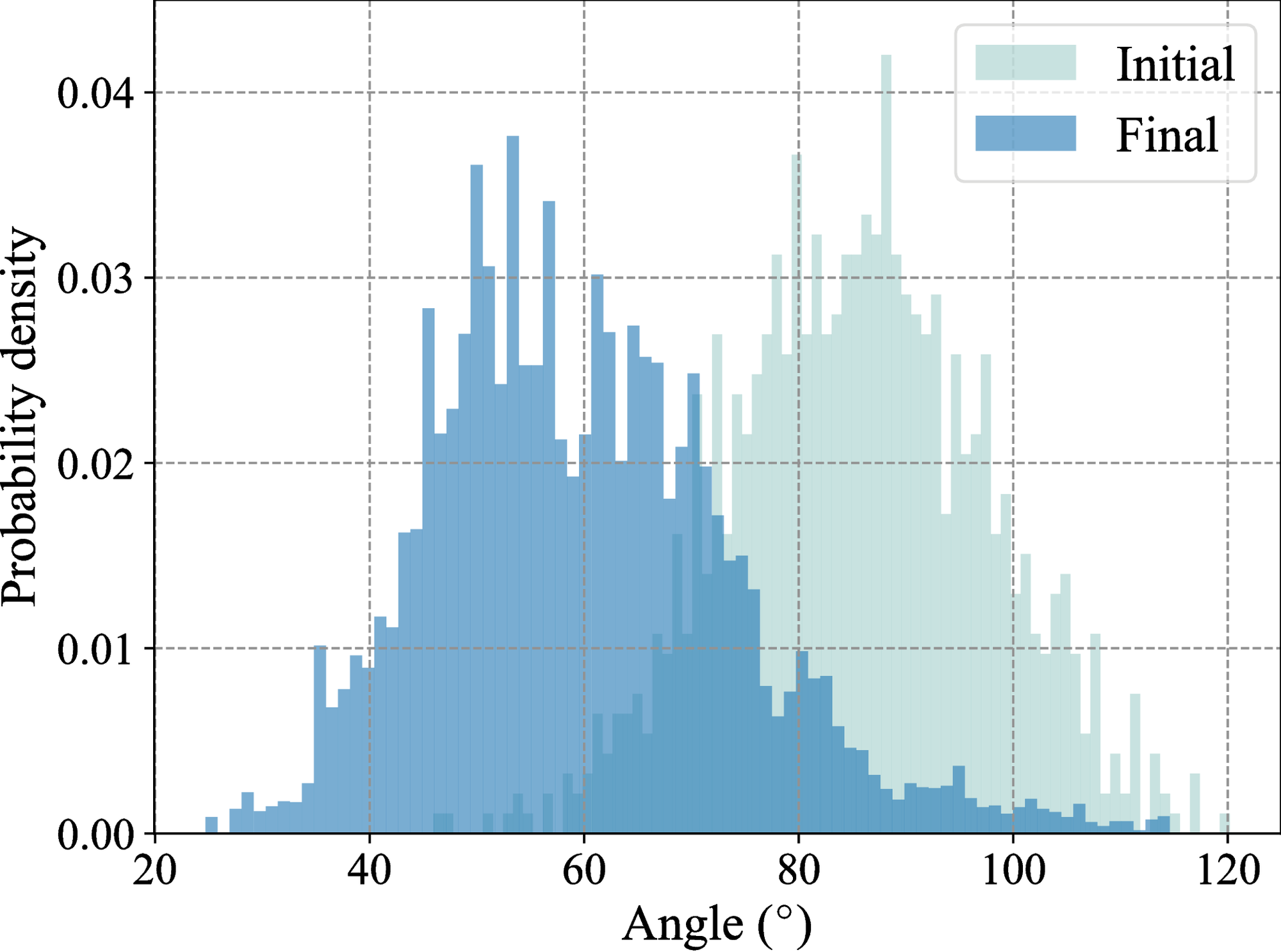
The above convergence behaviors are also linked with the histograms of the angles between the position and the decision across the population, see (9). Since the objective function of (36) is an inner product of the position \( p\) and the decision \( q\) , the angle between \( p\) and \( q\) is a useful indicator of the sign and the value of the inner product \( p^\top q\) . As shown in (9), the initial angles are largely distributed in \( [80^\circ, 100^\circ]\) , rendering the average population-wide affinity close to zero. The optimal solution returned by IPOPT and the solutions obtained by the vanilla algorithm (37) and our algorithm (39) all result in a final configuration wherein most angles fall into \( [40^\circ, 80^\circ]\) . Hence, the final average affinity is positive. Since the vanilla algorithm (37) focuses less on steering the distribution, in (10), there are relatively more final angles in \( [90^{\circ}, 115^{\circ}]\) , which accounts for a smaller affinity and a larger optimality gap as shown in (6). In contrast, the solution found by our algorithm (39) induces a nearly identical population-wide behavior as the ground truth.

(5.1) is concerned with affinity maximization involving continuous population distributions. In contrast, we now consider decision-making given discrete distributions lying in the probability simplex \( \Delta^{m} = \{p \in \mathbb{R}^m | 1^\top p = 1, 0 \leq p^i \leq 1, i=1,…,m\}\) , where \( m \in \mathbb{N}_{+}\) . This setting is motivated by a recommender system scenario, where a user selects a specific item (e.g., product, movie, or plan) from a set of candidates, and the choice model is characterized by a discrete distribution in \( \Delta^m\) . The recommender aims to optimize certain performance measures (e.g., of gain and diversity) by interacting with this user and adjusting its decision. This setting is also related to the multi-armed bandit problem, in that the user action described by a choice distribution \( p \in \Delta^m\) incurs performance feedback determined by the decision-maker.

We consider the following distribution dynamics

where \( p_k \in \Delta^m\) denotes the choice distribution at time \( k\) , \( q \in \mathbb{R}^m\) is a decision vector whose element represents, e.g., the price or loss of each item in a set, \( \lambda_1, \lambda_2 \in [0,1)\) are combination coefficients, and the \( i\) -th element of \( \operatorname{softmax}(-\epsilon q)\) is given by \( \exp(-\epsilon q^i)/\sum_{i=1}^{m} \exp(-\epsilon q^i)\) , where \( \epsilon > 0\) is a coefficient, and \( i=1,…,m\) . The term \( \operatorname{softmax}(-\epsilon q)\) gives a distribution consisting of probabilities proportional to the exponentials of \( -\epsilon q\) . One interpretation of this softmax operation is that an item \( i\) entailing a low price \( q^i\) is selected with a high probability. Similar to (34), the last term of (40) captures the persistent influence of the initial choice distribution. The steady-state distribution of (40) given a fixed decision \( q\) is

The recommender pursues maximizing its expected gain while preserving diversity, subject to certain budget requirements. This is formalized by the following problem

In problem (42), the first term \( p^\top q\) of the objective function represents the expected value given the steady-state discrete distribution \( p=h(q,p_0)\) , see also (41). This term indicates the expected price paid by the user, or conversely, the expected gain of the recommender. The second term of the objective is an entropy regularization with the coefficient \( \rho > 0\) , and its purpose is to promote diversity by favoring the distribution \( p\) with a high entropy. The remaining constraints of problem (42) specify budget requirements of the decision \( q\) , where \( b, \overline{q} > 0\) are constants.

Problem (42) involves the underlying distribution dynamics (40). An offline numerical solver hinges on an explicit and accurate model of (40) and requires sufficient waiting time for \( p_k\) to converge to its steady state \( p_\textup{ss}\) , which can be restrictive in practice. To solve problem (42) in an online fashion, the vanilla algorithm, which is of the style of performative prediction [16] and is oblivious to the composite problem structure, reads as follows

where \( \mathrm{Proj}_{\mathcal{C}}(\cdot)\) denotes the projection to the simplex \( \mathcal{C} = \{q \in \mathbb{R}^m | 1^\top q = b, 0 \leq q_i \leq \overline{q}\}\) , and \( \eta > 0\) is the step size. Another choice is the following derivative-free algorithm [57]

where \( \eta > 0\) is the step size, \( m\) is the dimension of \( q_k\) , \( \delta > 0\) is the smoothing parameter, \( v_k,v_{k-1}\) are independent random vectors uniformly sampled from the unit sphere in \( \mathbb{R}^m\) , and \( \Phi(q_k + \delta v_k, p_k)\) is the objective value evaluated at time \( k\) . Algorithm (44) exploits bandit feedback of the objective, and a similar version of (44) is adopted in [29, 41]. In contrast, our algorithm taking into account the composite structure due to decision dependence is

In (45), \( \eta>0\) is the step size, and the distribution sensitivity \( H^k\) (independent of \( p_k\) and \( p_0\) ) is

where the vector \( z_k \in \mathbb{R}^m\) is given by \( \exp(-\epsilon q_k)\) , and \( \operatorname{diag}(z_k)\) denotes a diagonal matrix with \( z_k\) as its diagonal elements. The ascent-based updates in (43), (44), and (45) are due to maximization in (42). Since the recommender interacts directly with a single user and does not require multiple samples, the update (45) differs slightly from (10), although both are grounded in the same principle.

In experiments, the vectors \( p\) for the choice distribution and the decision \( q\) are \( 100\) -dimensional vectors, i.e., \( m=100\) . In terms of the distribution dynamics (40), we set \( \lambda_1 = 0.2, \lambda_2 = 0.5\) , and \( \epsilon = 0.5\) . In problem (42), we set the regularization coefficient \( \rho = 0.1\) , the budget \( b = 250\) , and the upper bound \( \overline{q} = 5\) . For both algorithms (43) and (45), we select the step size \( \eta = 0.5\) . For the algorithm (44), we set \( \eta=0.1, \delta=2\) and run \( 20\) independent trials. We use IPOPT [56] to calculate the optimal value and the optimal point of problem (42) in an offline manner as benchmarks. However, as discussed earlier, numerical solvers can be restrictive in practice when the dynamics model (40) is inaccurate and real-time decision-making is necessary.

(13) shows the convergence results of online algorithms (43), (44), and (45) while interacting with the dynamics (40) to solve problem (42). The vanilla algorithm (43) is online in nature, and therefore it adapts to the changing distribution (40), eventually reaching a fixed-point solution. However, this algorithm suffers from significant sub-optimality, because it neglects the composite problem structure where the steady-state distribution is a function of the decision. The derivative-free algorithm (44) converges slowly due to the stochasticity of gradient estimates. In contrast, our algorithm (45) respects the composite structure by leveraging distribution sensitivities and regulating the shift of the choice distribution. Consequently, it attains a significantly higher solution accuracy. We remark that compared to (6) in (5.1), the curves of algorithms (43) and (45) in (13) do not exhibit stochastic oscillations, because we no longer resort to samples of a population distribution for mini-batch gradients.

The aforementioned difference in solution quality also causes the discrepancy in the evolution of the Wasserstein distances \( W_1(p_k, p_\textup{ss}(q^*))\) between the dynamic choice distribution \( p_k\) and the steady-state distribution \( p_\textup{ss}(q^*)\) induced by the optimal decision \( q^*\) via IPOPT . (16) illustrates such a difference in \( W_1(p_k, p_\textup{ss}(q^*))\) . Overall, these distances converge, thanks to the stable distribution dynamics (40) and the convergence of the algorithms to fixed decisions. We note that the vanilla algorithm (43) and the derivative-free algorithm (44) bring about biased final choice distributions, whereas our algorithm (45) drives the distribution to asymptotically converge to \( p_\textup{ss}(q^*)\) corresponding to the optimal decision. As pointed out earlier, this major difference is due to our algorithmic structure, which explicitly addresses the composite problem characteristic resulting from decision dependence.

The overarching idea is to analyze the coupled evolution of the distribution dynamics (3) and the algorithm (10). To this end, we first quantify the cumulative Wasserstein metric related to the distribution (3). Afterward, we focus on the iterative update of the algorithm (10) and synthesize the overall convergence measure, i.e., the average expected second moment of gradients.

We start with the following lemma that characterizes the cumulative sum of the squared Wasserstein distances between the distribution at each time and the corresponding steady-state distribution. It is built on (2) and further uses the condition (22) of the step size in (2), thereby exposing the true gradient \( \nabla \tilde{\Phi}(u_k)\) in the upper bound on this cumulative sum.

With (11) in hand, we are ready to prove (2).

The proof resembles what we have presented in (D.1). The key idea is to quantify the coupled evolution of optimization iterations and dynamic distributions. However, to establish convergence with high probability rather than in expectation, we will derive and exploit some tail bounds related to stochastic errors of gradients.

Throughout this subsection, we rely on the following decomposition

where \( e_k\) and \( \xi_k\) are given in (19) and (27), respectively. Specifically, \( e_k\) denotes the difference of expected gradients (i.e., \( \widehat{\nabla}^k \tilde{\Phi}(u_k)\) and \( \nabla \tilde{\Phi}(u_k)\) ) arising from the discrepancy between \( \gamma_k\) and \( \gamma_\textup{ss}(u_k)\) , and \( \xi_k\) indicates the stochastic noise in the mini-batch gradient \( \widehat{\nabla}_\textup{{mb}}^{k} \tilde{\Phi}(u_k)\) relative to its expectation \( \widehat{\nabla}^k \tilde{\Phi}(u_k)\) .

Along with the iteration (10), the stochastic noise \( \xi_k\) (27) exerts a cumulative influence on the accuracy of solutions. In the following lemma, we provide high-probability bounds on some cumulative quantities that involve \( \xi_k\) and are relevant to the overall convergence measure.

Similar to (11), the following lemma provides an upper bound on the cumulative squared Wasserstein distances. This cumulative sum quantifies the evolution of the distribution driven by the decision-maker. Due to the coupling between the distribution dynamics and the decision, the upper bound involves quantities related to gradients, which originate from optimization iterations.

We give the complete proof of (4). The key idea is to synthesize the convergence measure (i.e., the average second moment of gradients) from optimization iterations and the characterization of distribution dynamics in (13). We also leverage the high-probability bounds in (12).

We rely on the concentration of the empirical measure evaluated by Wasserstein distances [55]. Such a concentration is concerned with the closeness between \( \mu_d\) and \( \mu_d^N\) with high probability. Since \( \mu_d,\mu_d^N \in \mathcal{P}(\mathbb{R}^r)\) , we define \( W_1(\mu_d,\mu_d^N)\) as

The measure concentration argument is delineated in the following lemma.

The proof of (4) is as follows.

We first present a lemma of the angles between vectors involving conic combinations.

(15) formalizes the geometric intuition that if a vector lies in a conic region bounded by two vectors forming an acute angle, then this vector is closer to one of the boundary vectors than two boundary vectors are to each other. We provide the proof of (7) as follows.

Proof

We divide the proof into three parts. First, we prove the existence and uniqueness of the steady state \( p_\textup{ss}\) of the polarized dynamics (34). We then derive the steady-state sensitivity of (34). Finally, we quantify how the coefficients \( \lambda\) and \( \sigma\) in (34) influence the closeness between \( p_\textup{ss}\) and \( q\) (or \( -q\) ), an indicator of the steering ability of the decision-maker.

Existence and uniqueness of \( p_\textup{ss}\) : Note that the initial state \( p_0\) is nonzero, because \( \|p_0\|=1\) . We first address the special case in (3), i.e., \( p_0^\top q = 0\) . The dynamics (34) indicate that \( p_k = p_0 \neq 0, \forall k \in \mathbb{N}\) . Therefore, the steady state exists and is unique: it equals \( p_0\) . In another special case where \( p_0\) and \( q\) are parallel, the unique steady state is either \( q\) or \( -q\) , depending on \( \sigma\) , \( \|q\|\) , and if \( p_0\) and \( q\) are of the same or opposite direction.

We proceed to analyze the case in (4), i.e., \( p_0^\top q > 0\) and \( p_0\) and \( q\) are not parallel. Let \( \mathrm{sgn}(\cdot)\) denote the sign function, i.e., \( \mathrm{sgn}(x)\) equals \( -1\) , \( 0\) , or \( 1\) if \( x<0\) , \( x=0\) , or \( x>0\) , respectively. The initial condition satisfies \( \mathrm{sgn}(p_0^\top q) = 1\) . Suppose that for a particular \( k \in \mathbb{N}\) , \( p_k^\top q > 0\) holds. It follows from the dynamics (34) that

\[ \begin{equation} \mathrm{sgn}(p_{k+1}^\top q) = \mathrm{sgn}(\tilde{p}_{k+1}^\top q) = \mathrm{sgn}\left((\lambda + \sigma\|q\|^2)p_k^\top q + (1-\lambda)p_0^\top q\right) \stackrel{\text{(a.1)}}{=} 1, \end{equation} \]

(94)

where (a.1) uses the base case \( p_0^\top q > 0\) and the induction hypothesis \( p_k^\top q > 0\) . The above derivation is similar to [23, Proof of Propostion 1]. Hence, \( p_{k+1}^\top q > 0\) also holds. Therefore, for any \( k \in \mathbb{N}\) , \( p_k^\top q > 0\) , implying \( p_k\) is nonzero and that \( p_k\) and \( q\) always form an acute angle. Let \( p_k^+ \triangleq (1-\lambda)p_0 + \sigma \cdot (p_k^{\top} q) q\) be an intermediate vector. We now prove the following proposition on the angles related to \( p_k, p_{k+1}\) , and \( p_k^+\) illustrated by (17).

In the base case when \( k=0\) , \( p_0^+\) is a conic combination of \( p_0\) and \( q\) , and \( p_1\) is a conic combination of \( p_0\) and \( p_0^+\) . Therefore, (15) ensures that (1) holds. Suppose that (1) is true for a particular \( k \in \mathbb{N}\) . Because \( p_k\) and \( p_{k+1}\) are of unit norm and the angle between \( p_{k+1}\) and \( q\) is smaller than that between \( p_k\) and \( q\) , we know that \( 0 < p_{k}^\top q < p_{k+1}^\top q\) . Hence,

\[ p_{k+1}^+ = (1-\lambda)p_0 + \sigma\cdot (p_{k+1}^\top q)q \stackrel{\text{(a.1)}}{=} p_k^{+} + \underbrace{\sigma\cdot(p_{k+1}^\top q - p_k^\top q)}_{> 0} q, \]

where (a.1) uses the expression of \( p_k^+\) . Since \( p_{k+1}^+\) is a conic combination of \( p_k^+\) and \( q\) and the combination coefficients are positive, we know from (15) that the angle between \( p_{k+1}^+\) and \( q\) is smaller than that between \( p_k^+\) and \( q\) , which is further smaller than that between \( p_{k+1}\) and \( q\) (c.f. the induction hypothesis). Finally, \( p_{k+2}\) lies in the convex cone formed by \( p_{k+1}\) and \( p_{k+1}^+\) . Hence, (1) also holds true for \( k+1\) . Therefore, (1) is proved.

A consequence of (1) is that the angle between \( p_k\) and \( q\) is monotonically decreasing as \( k\) increases. Additionally, this angle is bounded from below by zero, because \( p_k\) always lies in the convex cone formed by \( p_0\) and \( q\) . The monotone convergence theorem ensures that there exists a unique steady state \( p_\textup{ss}\) , i.e., the limiting point of \( p_k\) .

The analysis for the case in (5) (i.e., \( p_0^\top q < 0\) ) is similar to the above analysis for (4) (i.e., \( p_0^\top q > 0\) ) by considering the convex cone formed by \( p_0\) and \( -q\) , or put differently, the angle between \( p_k\) and \( -q\) for different \( k\) .

Derivation of the steady-state sensitivity: The steady state of the dynamics (34) satisfies

\[ \begin{align} \tilde{p}_\textup{ss} &= \lambda p_\textup{ss} + (1-\lambda) p_0 + \sigma \cdot (p_\textup{ss}^{\top} q) q \triangleq \tilde{f}(p_\textup{ss},q,p_0), \\ p_\textup{ss} &= \frac{\tilde{p}_\textup{ss}}{\|\tilde{p}_\textup{ss}\|} = \frac{\tilde{f}(p_\textup{ss},q,p_0)}{\|\tilde{f}(p_\textup{ss},q,p_0)\|} \triangleq f(p_\textup{ss},q,p_0). \\\end{align} \]

(95.a)

We have proved that \( p_\textup{ss}\) (and also \( \tilde{p}_\textup{ss}\) ) are nonzero, see the reasoning about (94). Hence,

\[ \begin{align*} \nabla_q f(p_\textup{ss},q,p_0) &= \sigma \left[(p_\textup{ss}^\top q) I + p_\textup{ss} q^\top \right] \left(\frac{1}{\|\tilde{p}_\textup{ss}\|} I - \frac{\tilde{p}_\textup{ss} \tilde{p}^\top_\textup{ss}}{\|\tilde{p}_\textup{ss}\|^3} \right) = \frac{\sigma}{\|\tilde{p}_\textup{ss}\|} \left[(p_\textup{ss}^\top q) I + p_\textup{ss} q^\top \right] \left(I - p_\textup{ss} p_\textup{ss}^{\top}\right), \\ \nabla_p f(p_\textup{ss},q,p_0) &= (\lambda I + \sigma q q^\top) \frac{I - p_\textup{ss} p_\textup{ss}^\top}{\|\tilde{p}_\textup{ss}\|}. \end{align*} \]

We further apply (5) and obtain the steady-state sensitivity as follows

\[ \begin{align*} \nabla_q h(q,p_0) &= -\nabla_q f(p_\textup{ss},q,p_0) \left[\nabla_p f(p_\textup{ss},q,p_0) - I\right]^{-1} \\ &= - \sigma \left(p_\textup{ss}^\top q I + p_\textup{ss} q^\top\right)(I- p_\textup{ss} p_\textup{ss}^\top)\left[(\lambda I + \sigma q q^\top)(I-p_\textup{ss} p_\textup{ss}^\top) - \|\tilde{p}_\textup{ss}\| I\right]^{-1}. \end{align*} \]

The influence of coefficients: We quantify how the coefficients \( \lambda\) and \( \sigma\) in (34) determine the steering ability of the decision-maker, which is reflected by the angle \( \overline{\theta}\) between \( p_\textup{ss}\) and \( q\) (or \( -q\) ). We consider the case where \( p_0^\top q > 0\) and \( p_0\) and \( q\) are not parallel, and a similar reasoning applies to the case of \( p_0^\top q < 0\) . Let \( \phi \in (0,90^\circ)\) denote the angle between \( p_0\) and \( q\) . Note that \( p_0\) and \( p_\textup{ss}\) are of unit norm. Since \( p_\textup{ss}\) satisfies the fixed-point equation (95), the vector \( (1-\lambda) p_0 + \sigma\cdot(p_\textup{ss}^\top q) q\) (i.e., \( (1-\lambda) p_0 + \sigma\|q\|^2 \cos(\overline{\theta})q\) ) is collinear with \( p_\textup{ss}\) , see (18). While this illustration and the following analysis are for two-dimensional vectors, extensions can be derived for high-dimensional scenarios. We analyze the triangle in (18) and use the law of sines to obtain

\[ \frac{\sigma \|q\|^2 \cos(\overline{\theta})}{\sin(\phi-\overline{\theta})} = \frac{1-\lambda}{\sin(\overline{\theta})} ~ \stackrel{\text{(a.1)}}{\Longrightarrow} ~ \frac{\sin(2\overline{\theta})}{\sin(\phi-\overline{\theta})} = \frac{2(1-\lambda)}{\sigma \|q\|^2}, \]

where (a.1) invokes the double angle formula \( \sin(2\overline{\theta}) = 2\sin(\overline{\theta})\cos(\overline{\theta})\) . Note that \( \sin(2\overline{\theta})/\sin(\phi-\overline{\theta})\) is an increasing function of \( \overline{\theta}\) . The increase of \( \lambda \in [0,1]\) and \( \sigma > 0\) result in the decrease of \( \overline{\theta}\) , implying a stronger steering ability of the decision-maker.

[1] Lars Hellemo and Paul I Barton and Asgeir Tomasgard Decision-dependent probabilities in stochastic programs with recourse Computational Management Science 2018 15 3 369–395

[2] Fengqiao Luo and Sanjay Mehrotra Distributionally robust optimization with decision dependent ambiguity sets Optimization Letters 2020 14 8 2565–2594

[3] Beste Basciftci and Shabbir Ahmed and Siqian Shen Distributionally robust facility location problem under decision-dependent stochastic demand European Journal of Operational Research 2021 292 2 548–561

[4] Lauren Conger and Franca Hoffmann and Eric Mazumdar and Lillian Ratliff Strategic distribution shift of interacting agents via coupled gradient flows Advances in Neural Information Processing Systems 2023 36 45971–46006

[5] Cédric Villani Optimal Transport: Old and New Springer 2009 338

[6] Nicholas JA Harvey and Christopher Liaw and Yaniv Plan and Sikander Randhawa Tight analyses for non-smooth stochastic gradient descent Proceedings of the 32nd Conference on Learning Theory 2019 1579–1613

[7] Xiaoyu Li and Francesco Orabona A high probability analysis of adaptive SGD with momentum arXiv preprint arXiv:2007.14294 2020

[8] Liam Madden and Emiliano Dall'Anese and Stephen Becker High Probability Convergence Bounds for Non-convex Stochastic Gradient Descent with Sub-Weibull Noise Journal of Machine Learning Research 2024 25 241 1–36

[9] Shaojie Li and Yong Liu High probability guarantees for nonconvex stochastic gradient descent with heavy tails Proceedings of the International Conference on Machine Learning 2022 12931–12963

[10] Jan Hązła and Yan Jin and Elchanan Mossel and Govind Ramnarayan A geometric model of opinion polarization Mathematics of Operations Research 2024 49 1 251–277

[11] Jason Gaitonde and Jon Kleinberg and Éva Tardos Polarization in geometric opinion dynamics Proceedings of the 22nd ACM Conference on Economics and Computation 2021 499–519

[12] Alexander Shapiro and Darinka Dentcheva and Andrzej Ruszczynski Lectures on Stochastic Programming: Modeling and Theory SIAM 2021

[13] Jiashuo Jiang and Xiaocheng Li and Jiawei Zhang Online stochastic optimization with Wasserstein based non-stationarity arXiv preprint arXiv:2012.06961 2020

[14] Xuanyu Cao and Junshan Zhang and H Vincent Poor Online stochastic optimization with time-varying distributions IEEE Transactions on Automatic Control 2021 66 4 1840–1847

[15] Juan Perdomo and Tijana Zrnic and Celestine Mendler-Dünner and Moritz Hardt Performative prediction Proceedings of the International Conference on Machine Learning 2020 7599–7609

[16] Moritz Hardt and Celestine Mendler-Dünner Performative prediction: Past and future arXiv preprint arXiv:2310.16608 2023

[17] Sarah Dean and Evan Dong and Meena Jagadeesan and Liu Leqi Accounting for AI and Users Shaping One Another: The Role of Mathematical Models arXiv preprint arXiv:2404.12366 2024

[18] Nicolas Lanzetti and Florian Dörfler and Nicolò Pagan The impact of recommendation systems on opinion dynamics: Microscopic versus macroscopic effects Proceedings of the 62nd IEEE Conference on Decision and Control 2023 4824–4829

[19] Sanjay Chandrasekaran and Giulia De Pasquale and Giuseppe Belgioioso and Florian Dörfler Mitigating Polarization in Recommender Systems via Network-aware Feedback Optimization arXiv preprint arXiv:2408.16899 2024

[20] Anton V Proskurnikov and Roberto Tempo A tutorial on modeling and analysis of dynamic social networks. Part I Annual Reviews in Control 2017 43 65–79

[21] Mathieu Laurière and Sarah Perrin and Matthieu Geist and Olivier Pietquin Learning mean field games: A survey arXiv preprint arXiv:2205.12944 2022

[22] Vicky Chuqiao Yang and Daniel M Abrams and Georgia Kernell and Adilson E Motter Why are US parties so polarized? A "satisficing" dynamical model SIAM Review 2020 62 3 646–657

[23] Sarah Dean and Jamie Morgenstern Preference dynamics under personalized recommendations Proceedings of the 23rd ACM Conference on Economics and Computation 2022 795–816

[24] H.K. Khalil Nonlinear Systems Prentice Hall 2002

[25] John C Duchi and Hongseok Namkoong Learning models with uniform performance via distributionally robust optimization Annals of Statistics 2021 49 3 1378–1406

[26] Kuhn Distributionally Robust Optimization arXiv preprint arXiv:2411.02549 2024

[27] Celestine Mendler-Dünner and Juan Perdomo and Tijana Zrnic and Moritz Hardt Stochastic optimization for performative prediction Advances in Neural Information Processing Systems 2020 33 4929–4939

[28] Dmitriy Drusvyatskiy and Lin Xiao Stochastic optimization with decision-dependent distributions Mathematics of Operations Research 2023 48 2 954–998

[29] John P Miller and Juan C Perdomo and Tijana Zrnic Outside the echo chamber: Optimizing the performative risk Proceedings of the International Conference on Machine Learning 2021 7710–7720

[30] Meena Jagadeesan and Tijana Zrnic and Celestine Mendler-Dünner Regret minimization with performative feedback Proceedings of the International Conference on Machine Learning 2022 9760–9785

[31] Adhyyan Narang and Evan Faulkner and Dmitriy Drusvyatskiy and Maryam Fazel and Lillian J Ratliff Multiplayer performative prediction: Learning in decision-dependent games Journal of Machine Learning Research 2023 24 202 1–56

[32] Wenjing Yan and Xuanyu Cao Zero-regret performative prediction under inequality constraints Advances in Neural Information Processing Systems 2023 36 1298–1308

[33] Zachary Izzo and Lexing Ying and James Zou How to learn when data reacts to your model: Performative gradient descent Proceedings of the International Conference on Machine Learning 2021 4641–4650

[34] Qiang Li and Chung-Yiu Yau and Hoi-To Wai Multi-agent performative prediction with greedy deployment and consensus seeking agents Advances in Neural Information Processing Systems 2022 35 38449–38460

[35] Georgios Piliouras and Fang-Yi Yu Multi-agent performative prediction: From global stability and optimality to chaos Proceedings of the 24th ACM Conference on Economics and Computation 2023 1047–1074

[36] Joshua Cutler and Dmitriy Drusvyatskiy and Zaid Harchaoui Stochastic optimization under distributional drift Journal of Machine Learning Research 2023 24 147 1–56

[37] Killian Wood and Gianluca Bianchin and Emiliano Dall’Anese Online projected gradient descent for stochastic optimization with decision-dependent distributions IEEE Control Systems Letters 2022 6 1646–1651

[38] Killian Wood and Emiliano Dall’Anese Stochastic saddle point problems with decision-dependent distributions SIAM Journal on Optimization 2023 33 3 1943–1967

[39] Qiang Li and Hoi-To Wai State dependent performative prediction with stochastic approximation Proceedings of the International Conference on Artificial Intelligence and Statistics 2022 3164–3186

[40] Gavin Brown and Shlomi Hod and Iden Kalemaj Performative prediction in a stateful world Proceedings of the International Conference on Artificial Intelligence and Statistics 2022 6045–6061

[41] Mitas Ray and Lillian J Ratliff and Dmitriy Drusvyatskiy and Maryam Fazel Decision-dependent risk minimization in geometrically decaying dynamic environments Proceedings of the AAAI Conference on Artificial Intelligence 2022 36 8081–8088

[42] Debmalya Mandal and Stelios Triantafyllou and Goran Radanovic Performative reinforcement learning Proceedings of the International Conference on Machine Learning 2023 23642–23680

[43] Peter E Caines Mean field games Encyclopedia of Systems and Control Springer 2021 1197–1202

[44] Jiawei Huang and Niao He and Andreas Krause Model-Based RL for Mean-Field Games is not Statistically Harder than Single-Agent RL Proceedings of the International Conference on Machine Learning 2024

[45] Kai Cui and Heinz Koeppl Approximately solving mean field games via entropy-regularized deep reinforcement learning Proceedings of the International Conference on Artificial Intelligence and Statistics 2021 1909–1917

[46] Yongxin Chen and Tryphon T Georgiou and Michele Pavon Optimal transport in systems and control Annual Review of Control, Robotics, and Autonomous Systems 2021 4 89–113

[47] Antonio Terpin and Nicolas Lanzetti and Florian Dörfler Dynamic programming in probability spaces via optimal transport SIAM Journal on Control and Optimization 2024 62 2 1183–1206

[48] Andrea Simonetto and Emiliano Dall'Anese and Santiago Paternain and Geert Leus and Georgios B Giannakis Time-varying convex optimization: Time-structured algorithms and applications Proceedings of the IEEE 2020 108 11 2032–2048

[49] Adrian Hauswirth and Zhiyu He and Saverio Bolognani and Gabriela Hug and Florian Dörfler Optimization Algorithms as Robust Feedback Controllers Annual Reviews in Control 2024 57

[50] Hiroyasu Tsukamoto and Soon-Jo Chung and Jean-Jaques E Slotine Contraction theory for nonlinear stability analysis and learning-based control: A tutorial overview Annual Reviews in Control 2021 52 135–169

[51] Asen L Dontchev and R Tyrrell Rockafellar Implicit Functions and Solution Mappings Springer 2009 543 New York

[52] Léon Bottou and Frank E Curtis and Jorge Nocedal Optimization methods for large-scale machine learning SIAM Review 2018 60 2 223–311

[53] Saeed Ghadimi and Guanghui Lan Stochastic first-and zeroth-order methods for nonconvex stochastic programming SIAM Journal on Optimization 2013 23 4 2341–2368

[54] Ngoc Huy Chau and Éric Moulines and Miklos Rásonyi and Sotirios Sabanis and Ying Zhang On stochastic gradient Langevin dynamics with dependent data streams: The fully nonconvex case SIAM Journal on Mathematics of Data Science 2021 3 3 959–986

[55] Nicolas Fournier and Arnaud Guillin On the rate of convergence in Wasserstein distance of the empirical measure Probability Theory and Related Fields 2015 162 3 707–738

[56] Andreas Wächter and Lorenz T Biegler On the implementation of an interior-point filter line-search algorithm for large-scale nonlinear programming Mathematical Programming 2006 106 25–57

[57] Yan Zhang and Yi Zhou and Kaiyi Ji and Michael M Zavlanos A new one-point residual-feedback oracle for black-box learning and control Automatica 2022 136 110006

[58] Liviu Aolaritei and Nicolas Lanzetti and Hongruyu Chen and Florian Dörfler Distributional uncertainty propagation via optimal transport arXiv preprint arXiv:2205.00343 2022

[59] Songfu Cai and Fei Han and Xuanyu Cao Performative Control for Linear Dynamical Systems Advances in Neural Information Processing Systems 2024 37